图的数据结构
1. 图的概念
Section titled “1. 图的概念”学了离散数学和数据结构之后,对图的一个概念应该是要比较清晰的。从概念上说,应当是一个点集和一个边集。注意,这里的集合是严格的数学上的集合,即满足确定性、无序性、唯一性。当然,从中也可以看出有向图和无向图之间的区别了。
1.1. 图的数学表示
Section titled “1.1. 图的数学表示”1.1.1. 图
Section titled “1.1.1. 图”1.1.2. 点集
Section titled “1.1.2. 点集”1.1.3. 边集
Section titled “1.1.3. 边集”有向图和无向图的区别还是相当大的
a. 无向边集
Section titled “a. 无向边集”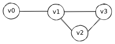
b. 有向边集
Section titled “b. 有向边集”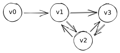
1.2. 图的连通性
Section titled “1.2. 图的连通性”这块应该都有所了解,此处从略。
2. 图的数据结构
Section titled “2. 图的数据结构”我知道前两部分的数据结构很拉,但谁不是从基础开始学起的呢。
2.1. 邻接矩阵
Section titled “2.1. 邻接矩阵”顾名思义,就是使用矩阵来存储。值得注意的是,无向图的矩阵是关于对角线对称的。
2.1.1. 图示
Section titled “2.1.1. 图示”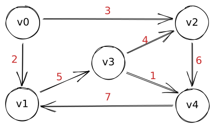
下面的矩阵表示从第 行到第 列的路径长度
2.1.2. 数据结构
Section titled “2.1.2. 数据结构”很明显,如果结点数为 ,邻接矩阵的数据结构就是用 的二维矩阵来表示的,这种数据结构适用于节点数量较少的稠密矩阵。此处没有路径直接用 0 来表示。
import numpy as np
class Edge:    def __init__(self, v_from, v_to, value):        self.v_from, self.v_to, self.value = v_from, v_to, value
class MatrixGraph(np.ndarray):    def __new__(cls, vexs: list, edges: list):        obj = np.zeros(shape=[len(vexs), len(vexs)], dtype=np.int32)        for edge in edges:            obj[edge.v_from, edge.v_to] = edge.value        return obj
m = MatrixGraph([0, 1, 2, 3, 4],                [Edge(0, 1, 2), Edge(1, 3, 5), Edge(0, 2, 3), Edge(2, 4, 6),                 Edge(3, 2, 4), Edge(3, 4, 1),Edge(4, 1, 7)])print(m)
2.2. 邻接链表
Section titled “2.2. 邻接链表”2.2.1. 图示
Section titled “2.2.1. 图示”
2.2.2. 数据结构
Section titled “2.2.2. 数据结构”可以看到,有一系列头节点,以及一系列跟随节点。头节点后面跟着的,就是从它直接可达的节点。这种数据结构适用于边数较少的稀疏图。
由于 python 没有指针,所以还是用 C++ 写吧
struct EdgeNode { int v_to; int value; EdgeNode* nextEdge;};struct VexNode { int data; EdgeNode* firstEdge;}class ALGraph { int vexnum, edgenum; vector<VexNode> adjList; // 顶点表public: ALGraph(vector<int>& vexs, vector<Edge>& edges) { EdgeNode* p; vexnum = vexs.size(); edgenum = edges.size(); adjList.resize(vexnum); for (int i = 0; i < vexnum; i++) { adjList[i].data = vexs[i]; // 顶点号 adjList.firstEdge = NULL; // 第一个后继 } for (int i = 0; i < edgenum; i++) { p = new EdgeNode; p->v_to = edges[i].v_to; p->value = edge[i].value; p->nextEdge = adjList[edges[i].v_from].firstEdge; // 插入表头 adjList[edges[i].v_from].firstEdge = p; } }};2.3. 链式前向星(用数组模拟邻接链表)
Section titled “2.3. 链式前向星(用数组模拟邻接链表)”来自某些网站的介绍
前向星是一种特殊的边集数组,我们把边集数组中的每一条边按照起点从小到大排序,如果起点相同就按照终点从小到大排序,并记录下以某个点为起点的所有边在数组中的起始位置和存储长度,那么前向星就构造好了。
再把上面的图拿下来。
2.3.1. 初步构建
Section titled “2.3.1. 初步构建”此时,我们构造这样的数据结构
struct Edge { int to, next, dist;};Edge e[E];int cnt, vexnum, edgenum;int head[N];同时,加边的方式也变了很多
void addEdge(int from, int to, int dist) { cnt++; e[cnt].dist = dist; // 边的权重 e[cnt].to = to; // 指向的下一个顶点 e[cnt].next = head[from]; // 第 cnt 条边的下一条边的序号 head[from] = cnt; // head[i] 保存的是以 i 为起点的所有边中编号最大的那个}// head 初始化为 -1乍一看,是个人都很难看懂,所以需要一番仔细分析。
在结构体 Edge 中,理所应当的存储的就是边的信息,而 head 数组,就是为辅助它而生的。我们先尝试按照代码逻辑进行加边的操作。(在本例中,其实还不怎么能看得出来)
| cnt | 1 | 2 | 3 | 4 | 5 | 6 | 7 |
|---|---|---|---|---|---|---|---|
| dist | 2 | 5 | 3 | 6 | 4 | 1 | 7 |
| from | 1 | 2 | 1 | 3 | 4 | 4 | 5 |
| to | 2 | 4 | 3 | 5 | 3 | 5 | 2 |
| next | -1 | -1 | 1 | -1 | -1 | 5 | -1 |
| head[from] | 2 | 3 | 4 | 6 | 7 |
在取出边的时候是怎么取的呢
void show(){ int i, t; for (int i = 1; i <= vexnum; i++) { t = head[i]; while (t != -1) { cout << i << "--->" << e[t].to << ", dist: " << e[t].dist << endl; t = e[t].next; } }}控制台输出
1--->3, dist: 31--->2, dist: 22--->4, dist: 53--->5, dist: 64--->5, dist: 14--->3, dist: 45--->2, dist: 72.3.2. 根据代码与流程进行分析
Section titled “2.3.2. 根据代码与流程进行分析”外层循环表示有多少个节点,也就是说,我们还是从节点出发,然后再判断这个节点的出度为多少。而出度的判断,则需要用到 next 了。
首先,在这里的示例中,head[i] 的值与节点的编号看似是相同的,但其实可以发现,每当遇到一个来源相同的节点,head 在此处的值都会被覆盖一次。也就是说,head[from] 中会记录以 from 为起点的边的最大索引。
另外,这里还有一个被忽略的点,即在建图完成之后,只有索引值最低的 head 元素是有效的,也就是说,上表中 from 值相同的 head 元素,在后续操作时,只有“第一个”head 是有用的,在本例中其实有点看不出来,在节点和边较多的图中能体现的比较明显
而在循环中的 t = e[t].next 这一步极为关键,上次看到这个式子还是在 KMP 算法中。当时,j = next[j] 的意思是,将当前不匹配的索引前向丢弃(这一块有所遗忘,可能还需要复习一下)。在这里,e[cnt].next = head[from] 的 next 中记录了上一次遇到的,以 from 为起始节点的那条边的索引。
另外,光是看这么一个式子,即 t = e[t].next,其实就有链表的一重意思在里面了,但还不完全是链表。
现在再来看内层的循环,根据上面关于 head 的讨论,t=head[i] 这句的含义为,取出以 i 为起始节点的索引值最大的一条边(即起点为 i 的,最后一次输入的边)。因此,在输出过程中,会将最后一条以 i 为起始的边先输出出来。
而后进行的 t = e[t].next 操作,即取出同样以 i 为起始的倒数第二条边。因此,next 其实不如说是 forward,也就是说,这种取出的方式,其实是按照输入的反向进行输出的。最后,当 t 的值为 -1 时,也就是说,以 i 为起始的节点没有边了,那么就停止。
至此,我个人对于链式前向星这一存储图的数据结构的第一次系统整理,让我对数据结构有了一番新的认识。
// 主函数(加边)int main(){ cnt = 0; memset(e, 0, sizeof e); memset(head, -1, sizeof head); cin >> vexnum >> edgenum; int from, to, dist; while (edgenum--) { cin >> from >> to >> dist; addEdge(from, to, dist); } show(); return 0;}2.3.3. 使用样例
Section titled “2.3.3. 使用样例”我们不妨就拿这种数据结构尝试写一下拓扑排序吧。
#include <iostream>#include <queue>using namespace std;const int N = 10005;struct Edge{ int to, next;} e[N];int head[N];int indeg[N];int cnt, n, m;void addEdge(int from, int to){ cnt++; e[cnt].to = to; // 下一个节点编号 e[cnt].next = head[from]; // 下(前)一条边的序号 head[from] = cnt; indeg[to]++; // 某个节点的入度增加}void topo(queue<int> &q){ for (int i = 1; i <= n; i++) if (indeg[i] == 0) q.push(i); // 入度为 0 的节点入队 while (!q.empty()) { int tmp = q.front(); // 取出一个入度为 0 的节点 q.pop(); for (int t = head[tmp]; t != -1; t = e[t].next) { int vex_to = e[t].to; // 找到它的一个目标节点 cout << tmp << "-->" << vex_to << endl; // 输出它的路径 indeg[vex_to]--; // 目标节点的入度减一 if (indeg[vex_to] == 0) // 如果入度为 0,即没有前驱节点了 q.push(vex_to); // 那么将这一个节点入队 } }}int main(){ int x, y; cin >> n >> m; for (int i = 0; i <= n; i++) { head[i] = -1, indeg[i] = 0; // 初始化需要用到的元素 } for (int i = 1; i <= m; i++) { cin >> x >> y; addEdge(x, y); // 加边 } queue<int> q; topo(q); return 0;}2.4. multi_map 存储
Section titled “2.4. multi_map 存储”在 map 数据结构中,它不允许有相同的键,但是 multi_map 却能够重复的添加相同的键。因此,我们可以使用它来存储图的结构,其 first 和 second 分别对应一条边的起点和终点。
multi_map<int, int> m;void buildGraph(int n){ int x, y; for (int i = 0; i < n; i++) { cin >> x >> y; m[x] = y; // 无向图 m[y] = x; // 需要双向赋值 }}void outputGraph(){ for (auto it = m.begin(); it != m.end(); it++) { cout << it->first << "-->" << it->second << endl; }}